18. Non-Conjugate Priors#
GPU
This lecture was built using a machine with access to a GPU — although it will also run without one.
Google Colab has a free tier with GPUs that you can access as follows:
Click on the “play” icon top right
Select Colab
Set the runtime environment to include a GPU
In addition to what’s in Anaconda, this lecture will need the following libraries:
!pip install numpyro jax arviz
18.1. Overview#
This lecture is a sequel to Two Meanings of Probability.
In that lecture we adopted a beta prior for the unknown probability \(\theta\) of a coin landing heads, together with a binomial likelihood.
That prior and likelihood form a conjugate pair: applying Bayes’ law returns a posterior of the same family as the prior — again a beta distribution.
Conjugacy is convenient because it delivers a posterior in closed form.
But a person’s prior beliefs are their own business, and in general they will not happen to be conjugate to the likelihood.
When the prior and likelihood are not conjugate, the posterior usually has no closed form, and we must approximate it numerically.
This lecture introduces two widely used ways to do that, both implemented in the probabilistic programming library NumPyro:
Markov chain Monte Carlo (MCMC) — construct a Markov chain whose stationary distribution is the posterior, then sample from it. We use the No-U-Turn Sampler (NUTS), a state-of-the-art form of Hamiltonian Monte Carlo.
Variational inference (VI) — replace sampling with optimization: search within a tractable family of distributions for the member closest to the posterior.
Note
We treat NUTS as a black box in this lecture.
In brief, it is a form of Hamiltonian Monte Carlo, which is itself a version of the Metropolis–Hastings algorithm: it proposes candidate draws and accepts or rejects them so that the resulting Markov chain has the posterior as its stationary distribution.
What distinguishes it from a basic Metropolis–Hastings sampler is that its proposals are built from gradient (derivative) information about the log-posterior, which lets the chain move efficiently through the parameter space; NUTS additionally tunes the length of each proposed move automatically.
For a more advanced introduction to MCMC and the Metropolis–Hastings algorithm, see this lecture.
Our plan is:
Confirm that MCMC reproduces the conjugate beta posterior that we can compute analytically — this validates the machinery on a problem whose answer we already know.
Replace the beta prior with several non-conjugate priors and approximate each posterior with MCMC.
Introduce variational inference and compare it with MCMC.
Let us start with some imports.
import numpy as np
import matplotlib.pyplot as plt
import scipy.stats as st

import jax.numpy as jnp
from jax import random

import numpyro
import numpyro.distributions as dist
from numpyro.infer import MCMC, NUTS, SVI, Trace_ELBO
from numpyro.infer.autoguide import AutoNormal
from numpyro.optim import Adam

import arviz as az
18.2. The coin-flipping model#
As in Two Meanings of Probability, a coin lands heads (\(Y=1\)) with probability \(\theta\) and tails (\(Y=0\)) with probability \(1-\theta\).
If we flip the coin \(n\) times, the number of heads \(k\) has the binomial distribution
We treat \(\theta\) as a random variable with a prior density \(p(\theta)\), and we want the posterior
18.2.1. Generating data#
We simulate a sequence of coin flips from a coin whose true (but unknown to the analyst) probability of heads is \(\theta = 0.4\).
def simulate_coin_flips(θ=0.4, n=20, seed=1234):
    "Flip a coin n times; return an array of 0s (tails) and 1s (heads)."
    rng = np.random.default_rng(seed)
    return (rng.random(n) < θ).astype(int)

data = simulate_coin_flips()
k, n = int(data.sum()), len(data)
k, n
(9, 20)
We deliberately use a small sample (\(n = 20\)).
The reason is that the prior matters most when data are scarce.
With a large sample the likelihood dominates and almost any reasonable prior leads to the same posterior — exactly the concentration we saw in Two Meanings of Probability.
A modest \(n\) keeps the influence of the prior visible, which is what we want to study here.
18.2.2. Specifying the model in NumPyro#
For most readers this will be a first encounter with NumPyro, whose style takes some getting used to.
To use it we describe our probability model as a Python function — which, a little confusingly, NumPyro calls a model.
Such a function does not compute anything when called, and it does not return the posterior.
Instead it is a declaration of the generative story for the data: which quantities are random, how they are distributed, and how the data depend on them.
An inference algorithm — such as the NUTS sampler below — then reads this declaration and works out the posterior for us.
Inside a model, every random quantity is introduced by a call to numpyro.sample, and the keyword obs decides its role:
numpyro.sample("θ", prior)introduces a latent (unobserved) variable named"θ", drawn fromprior— a quantity we wish to infer.numpyro.sample("k", dist.Binomial(n, θ), obs=k)introduces an observed variable: the keywordobs=kpins it to the data, which is how the likelihood \(p(k \mid \theta)\) enters.
The string names ("θ" and "k") are the labels NumPyro uses to keep track of the variables; we will use them later to pull the posterior draws back out.
We write a single model that takes the prior distribution as an argument, so we can reuse it unchanged for every prior we consider — conjugate or not.
def binomial_model(prior, k, n):
    "Binomial likelihood with a caller-supplied prior on θ."
    θ = numpyro.sample("θ", prior)
    numpyro.sample("k", dist.Binomial(n, θ), obs=k)
Notice that binomial_model returns nothing, and that we never call it ourselves.
Instead we hand it to an inference algorithm, which supplies the arguments and traces the two sample statements to assemble the posterior.
We also write a small helper that runs NUTS on a given model and returns the fitted sampler.
We request four chains so that we can check convergence below, and run them with chain_method="vectorized", which evaluates all chains together on a single device — so the same code runs unchanged on a CPU or a GPU.
def run_nuts(model, *args, seed=0, num_warmup=1000, num_samples=4000, num_chains=4):
    "Sample a NumPyro model with the NUTS sampler."
    mcmc = MCMC(
        NUTS(model),
        num_warmup=num_warmup,
        num_samples=num_samples,
        num_chains=num_chains,
        chain_method="vectorized",
        progress_bar=False,
    )
    mcmc.run(random.key(seed), *args)
    return mcmc
NumPyro is built on JAX, which treats randomness explicitly: rather than relying on a global random state, each run needs its own PRNG key, created here with random.key(seed).
(This is why we used NumPy’s generator to make the data above but JAX keys here.)
run_nuts is deliberately generic: it samples whatever model we pass and forwards the extra arguments (*args) on to that model through mcmc.run. We always call it as run_nuts(binomial_model, prior, k, n), so prior, k, and n reach binomial_model unchanged — there is only ever the one prior.
18.3. MCMC reproduces the conjugate posterior#
Before trusting MCMC on hard problems, let us check it on an easy one.
With a \(\text{Beta}(\alpha_0, \beta_0)\) prior the posterior is known analytically (see Two Meanings of Probability):
We take \(\alpha_0 = \beta_0 = 2\) and sample the posterior with NUTS.
α0, β0 = 2.0, 2.0
mcmc = run_nuts(binomial_model, dist.Beta(α0, β0), k, n)
Before looking at the posterior we should check that the sampler has done its job.
Unlike the independent draws we are used to, MCMC returns a dependent sequence — a Markov chain — whose early draws still remember where the chain started.
We can trust the output only once the chain has “forgotten” its starting point and settled into its stationary distribution, which by construction is the posterior we want.
As a safeguard we ran four chains from different random starting points (num_chains=4 in run_nuts) and now check that they agree with one another.
ArviZ is a companion library for examining the output of Bayesian samplers.
The function az.from_numpyro repackages our NumPyro results into ArviZ’s standard data structure, and az.summary prints a table of per-parameter summaries and convergence diagnostics.
idata = az.from_numpyro(mcmc)
az.summary(idata, var_names=["θ"])
| mean | sd | eti89_lb | eti89_ub | ess_bulk | ess_tail | r_hat | mcse_mean | mcse_sd | |
|---|---|---|---|---|---|---|---|---|---|
| θ | 0.461 | 0.1 | 0.3 | 0.62 | 5861 | 7337 | 1.00 | 0.0013 | 0.00088 |
Two columns of this table are convergence diagnostics worth understanding.
r_hat(the Gelman–Rubin statistic) compares the spread of the draws within each chain to the spread between chains. If the chains have all converged to the same distribution these two match andr_hatis close to \(1.0\); values above roughly \(1.01\) warn that the chains disagree and the draws cannot yet be trusted.ess_bulkandess_tailreport the effective sample size. Because consecutive MCMC draws are correlated, a chain of length \(N\) carries less information than \(N\) independent draws would; the effective sample size estimates how many independent draws it is worth (in the bulk and in the tails of the distribution respectively). Larger is better.
Here r_hat is essentially \(1.0\) and the effective sample sizes run into the thousands, so the chains have mixed well.
A trace plot gives a visual check of the same thing.
ArviZ’s plot_trace draws two panels for each parameter: on the right, the sampled value against the iteration number (one coloured line per chain); on the left, a density estimate of the draws from each chain.
Well-mixed chains look like stationary noise on the right — a fuzzy, flat band, with the chains overlapping rather than drifting or wandering — and their densities on the left lie almost on top of one another.
az.plot_trace(idata, var_names=["θ"])
plt.tight_layout()
plt.show()
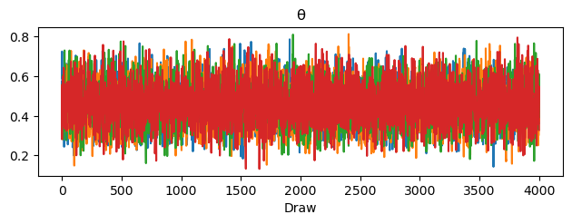
Our chains pass both checks, so we can trust the draws and turn to the posterior itself.
Now we compare the MCMC posterior with the analytical beta posterior.
θ_grid = np.linspace(0.001, 0.999, 500)
samples = np.asarray(mcmc.get_samples()["θ"])

fig, ax = plt.subplots()
ax.hist(samples, bins=50, density=True, alpha=0.4,
        label="MCMC posterior")
ax.plot(θ_grid, st.beta(α0 + k, β0 + n - k).pdf(θ_grid),
        'k-', lw=2, label="analytical posterior")
ax.plot(θ_grid, st.beta(α0, β0).pdf(θ_grid),
        'C1--', lw=2, label="prior")
ax.set_xlabel(r"$\theta$")
ax.legend()
plt.show()
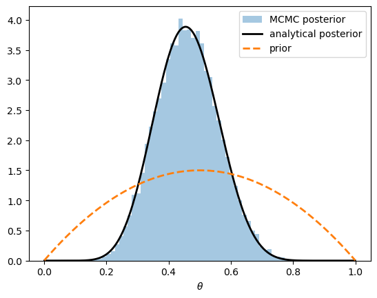
The histogram of MCMC draws sits right on top of the analytical posterior density.
The sampler works, so we can rely on it for priors that have no closed-form posterior.
18.4. Non-conjugate priors#
We now keep the binomial likelihood and the same data, but replace the beta prior with priors that are not conjugate to it.
For each prior the recipe is identical:
describe the prior and build it as a NumPyro distribution,
pass it to
binomial_modeland run NUTS,plot the prior against the resulting posterior.
The following helper draws a prior density and the posterior samples on the same axes.
def plot_prior_posterior(prior, samples, title=""):
    "Overlay a prior density and posterior MCMC draws for θ on [0, 1]."
    grid = jnp.linspace(0.001, 0.999, 500)
    # mask the density to the prior's support: dist.Uniform.log_prob
    # returns its constant value even outside [low, high]
    in_support = np.asarray(prior.support(grid))
    prior_pdf = np.where(in_support, np.exp(np.asarray(prior.log_prob(grid))), 0.0)

    fig, ax = plt.subplots()
    ax.hist(np.asarray(samples), bins=50, density=True, alpha=0.4,
            label="posterior (MCMC)")
    ax.plot(np.asarray(grid), prior_pdf, 'C1--', lw=2, label="prior")
    ax.set_xlabel(r"$\theta$")
    ax.set_xlim(0, 1)
    ax.legend()
    if title:
        ax.set_title(title)
    plt.show()
18.4.1. A uniform prior#
The simplest non-conjugate prior is uniform: the analyst regards every value of \(\theta\) in some interval as equally likely.
A uniform prior on all of \([0, 1]\) expresses indifference.
Because its density is constant, the posterior is then proportional to the likelihood alone.
mcmc_flat = run_nuts(binomial_model, dist.Uniform(0.0, 1.0), k, n)
plot_prior_posterior(dist.Uniform(0.0, 1.0),
                     mcmc_flat.get_samples()["θ"],
                     title="flat uniform prior")
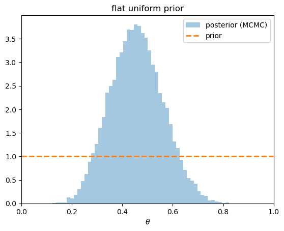
The posterior is centered near the sample frequency \(k/n\), just as the likelihood is.
Now suppose instead that the analyst is convinced the coin favors heads, and places a uniform prior on \([0.5, 0.95]\).
This prior assigns zero density to the region around the true value \(\theta = 0.4\).
mcmc_restr = run_nuts(binomial_model, dist.Uniform(0.5, 0.95), k, n)
plot_prior_posterior(dist.Uniform(0.5, 0.95),
                     mcmc_restr.get_samples()["θ"],
                     title="restrictive uniform prior")
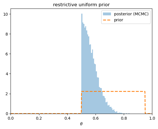
The posterior cannot put mass where the prior is zero, so it piles up against the lower boundary \(0.5\) — as close to the data as the prior permits.
This is a vivid warning: a prior that rules out the truth can never be overturned by data, no matter how much we collect.
18.4.2. A truncated log-normal prior#
A uniform prior is flat. A more realistic prior is smooth and asymmetric.
A convenient choice on \([0, 1]\) is a truncated log-normal: take \(Z \sim N(\mu, \sigma)\) truncated to \(Z \le 0\), and set \(\theta = e^{Z}\), which then lies in \((0, 1]\).
NumPyro builds this by feeding a TruncatedNormal through an ExpTransform.
def truncated_lognormal(μ, σ):
    "Log-normal distribution truncated to the unit interval (0, 1]."
    base = dist.TruncatedNormal(loc=μ, scale=σ, low=-jnp.inf, high=0.0)
    return dist.TransformedDistribution(base, dist.transforms.ExpTransform())

prior_ln = truncated_lognormal(0.0, 1.0)
mcmc_ln = run_nuts(binomial_model, prior_ln, k, n)
plot_prior_posterior(prior_ln, mcmc_ln.get_samples()["θ"],
                     title="truncated log-normal prior")
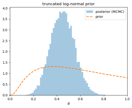
The prior favors smaller values of \(\theta\), but with \(\sigma = 1\) it is diffuse, so the likelihood pulls the posterior toward the sample frequency.
We keep mcmc_ln — we will compare it with variational inference below.
18.4.3. A truncated Laplace prior#
Our final prior has a sharp, non-smooth peak.
A Laplace density \(\propto e^{-|\theta - \mu| / b}\) has a kink at its center \(\mu\), expressing a strong belief that \(\theta\) sits near \(\mu\) while still allowing for surprises in the tails.
We truncate it to \([0, 1]\) and center it at \(0.5\).
def truncated_laplace(μ, b):
    "Laplace distribution truncated to the unit interval [0, 1]."
    return dist.TruncatedDistribution(dist.Laplace(μ, b), low=0.0, high=1.0)

prior_lp = truncated_laplace(0.5, 0.1)
mcmc_lp = run_nuts(binomial_model, prior_lp, k, n)
plot_prior_posterior(prior_lp, mcmc_lp.get_samples()["θ"],
                     title="truncated Laplace prior")
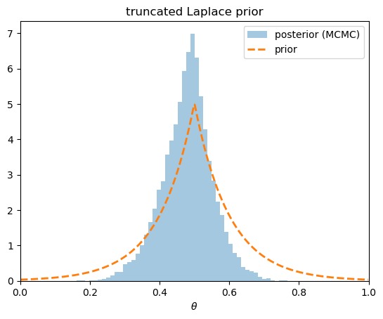
The spiked prior tugs the posterior toward \(0.5\), away from the sample frequency near \(0.4\).
The pull is gentle here because the prior, though peaked, is not very tight; with a smaller \(b\) it would dominate the modest sample.
NUTS handles the kink in the prior without any special tuning — a practical advantage of gradient-based samplers paired with automatic differentiation.
18.5. Variational inference#
MCMC approximates the posterior by sampling from it.
Variational inference (VI) takes a different route: it turns posterior approximation into an optimization problem.
We restrict attention to a tractable family of densities \(q_\phi(\theta)\) — the guide — indexed by parameters \(\phi\), and we search for the member of that family closest to the posterior.
18.5.1. Why variational inference?#
If NUTS already returns accurate posteriors, why introduce another method?
The answer is scale.
MCMC evaluates the likelihood over the entire dataset at every step, and the number of steps it needs tends to grow with the dimension of the parameter.
For large datasets or high-dimensional models — for instance the hierarchical models and neural networks common in machine learning — this can become too slow to be practical.
Variational inference scales much better, because the objective (the ELBO, introduced below) can be maximized with stochastic gradients computed on small random subsets of the data — the same machinery that trains deep learning models.
It also yields a compact parametric approximation that is cheap to store and to draw from afterwards.
The price is accuracy: VI returns only the best fit within the guide family, and it can understate uncertainty.
As a rule of thumb, prefer MCMC when you need an accurate posterior and the problem is small enough to afford it, and VI when the model is too large for MCMC or a fast, approximate answer is good enough.
18.5.2. The evidence lower bound#
Let the prior be \(p(\theta)\) and the likelihood be \(p(Y \mid \theta)\), where \(Y\) denotes the observed data (here the head count \(k\)).
By Bayes’ rule,
where
The integral in (18.1) is the troublesome one: in the non-conjugate case it has no closed form.
We measure the discrepancy between the guide \(q_\phi(\theta)\) and the posterior with the Kullback–Leibler (KL) divergence
and we choose \(\phi\) to minimize it.
The KL divergence still involves the intractable posterior, but we can rearrange it. Using \(p(\theta \mid Y) = p(\theta, Y) / p(Y)\),
where the last line uses \(\int q_\phi(\theta)\, d\theta = 1\). Rearranging,
The marginal likelihood \(\log p(Y)\) on the left does not depend on \(\phi\).
Hence minimizing the KL divergence is equivalent to maximizing the second term, the evidence lower bound (ELBO):
Because \(D_{KL} \ge 0\), the ELBO is a lower bound on \(\log p(Y)\) — hence its name.
Crucially, (18.2) involves only the joint density \(p(\theta, Y) = p(Y \mid \theta)\, p(\theta)\), which we can evaluate, not the intractable normalizing constant \(p(Y)\).
The expectation can be estimated by sampling from \(q_\phi\), and \(\phi\) improved by gradient ascent — this is stochastic variational inference (SVI).
18.5.3. Implementing SVI in NumPyro#
We need a guide \(q_\phi\).
The simplest choice is an autoguide: NumPyro inspects the model and automatically constructs a guide for us.
AutoNormal places an independent normal distribution on each latent variable, transformed to respect its support — here, to keep \(\theta\) inside \((0, 1)\).
We apply SVI to the truncated log-normal model from above and maximize the ELBO with the Adam optimizer.
guide = AutoNormal(binomial_model)
optimizer = Adam(step_size=0.01)
svi = SVI(binomial_model, guide, optimizer, loss=Trace_ELBO())

svi_result = svi.run(random.key(0), 5000, prior_ln, k, n, progress_bar=False)
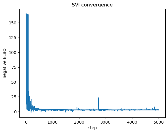
SVI maximizes the ELBO; equivalently, it minimizes its negative, which is the reported loss.
A loss curve that flattens out indicates convergence.
fig, ax = plt.subplots()
ax.plot(svi_result.losses)
ax.set_xlabel("step")
ax.set_ylabel("negative ELBO")
ax.set_title("SVI convergence")
plt.show()
18.5.4. Comparing VI with MCMC#
To assess the approximation, we draw samples from the fitted guide and compare them with the NUTS posterior for the same (log-normal-prior) model.
vi_samples = guide.sample_posterior(
    random.key(1), svi_result.params, sample_shape=(4000,)
)["θ"]
nuts_samples = mcmc_ln.get_samples()["θ"]

fig, ax = plt.subplots()
ax.hist(np.asarray(nuts_samples), bins=50, density=True, alpha=0.4,
        label="MCMC (NUTS)")
ax.hist(np.asarray(vi_samples), bins=50, density=True, alpha=0.4,
        label="VI (AutoNormal)")
ax.set_xlabel(r"$\theta$")
ax.legend()
plt.show()
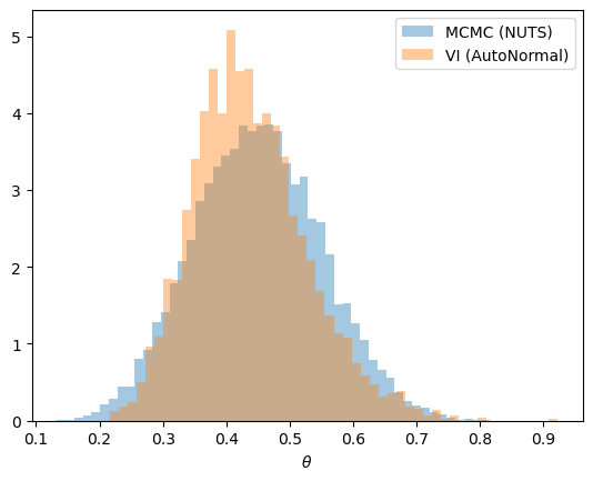
The two approximations broadly agree on the location and spread of the posterior.
They need not agree perfectly.
MCMC samples the true posterior (up to Monte Carlo error), whereas VI reports the best fit within its guide family.
A mean-field normal guide is symmetric on the transformed scale and can miss skewness or heavy tails in the true posterior.
The trade-off is one of cost against fidelity: VI replaces sampling with optimization and is often much faster in high dimensions, but it delivers an approximation whose quality is capped by the flexibility of the guide.
18.6. Where to next#
This lecture showed how to compute posteriors when prior and likelihood are not conjugate, using NUTS and stochastic variational inference in NumPyro.
The same tools carry over to richer models.
The lectures Posterior Distributions for AR(1) Parameters and Forecasting an AR(1) Process apply NumPyro to Bayesian estimation and forecasting of autoregressive time series, where the parameter is a vector and conjugate analysis is unavailable.